Navigation:  Special computations > ColorBox

This object computes the variation of the color coordinates a* and b* due to thickness fluctuations. The parameters of the computation (obtained with the Edit command) are the following:

 

 

Select the spectrum the color of which you want to investigate and enter the number of iterations that are to be used in the computations - in this case you will get 100 values for a* and b*. If you activate the checkbox Automatic re-computation all 100 values are computed whenever you change a model parameter (by a slider movement, for example). Since this means to re-compute the whole model 100 times the program may react slow with this option activated. If disabled the data are computed on demand only, i.e. by a click on the corresponding view object (see below).

 

If you check the option Compute average spectrum the average spectrum is computed during a re-computation. In order to visualize the average spectrum you have to generate a view element of type Field view in the list of view elements and then assign the colorbox object to the new field view object by drag and drop. The field view object will take the assigned colorbox object as source and display its average spectrum.

 

If you like you can define a rectangle in the a*-b* plane to visualize the tolerated area of color (target box). The rectangle is drawn in the color specified by the RGB values in the dialog.

 

Activating the option Display color background draws a colored background indicating the color impression for the various positions in color space. With the settings shown above this background is drawn using 2500 little rectangles (50 by 50).

 

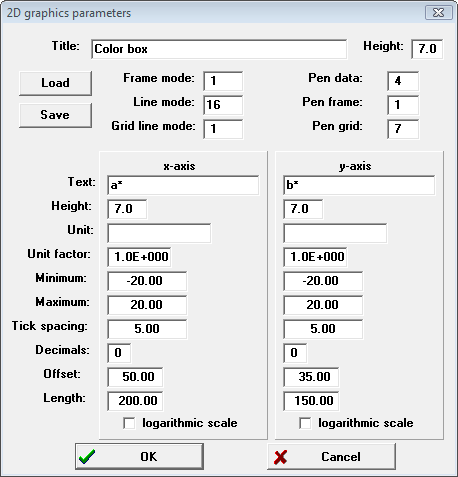
The ColorBox graph of b* vs. a* can be shown in a view object. The graphics parameters are set in the following dialog:

 

 

If you have checked the option 'Compute average spectrum' a second graphics dialog will open up which sets the parameters for the visualization of the average spectrum in the field view object (see above).

 

Since the color box graph will show a cloud of points you should use a 'line mode' for individual points (11, 12, 13, 14 or 16, see graphics course) but no continuous lines connecting the points.

 

In order to really see the color box drag the object from the list of special computations either directly to the main window of SCOUT or the list of the current view objects. In a view, a color box looks like this:

 

 

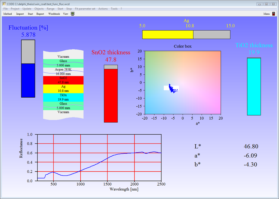
A mouse click on the object in a view activates the re-computation of the object's data (unless you activated the option of automatic re-computation).

 

The example above shows a configuration which allows to regulate the strength of the thickness fluctuation of all layers by the slider on the left side. If automatic re-computation for the ColorBox object is selected, you can instantly watch the cloud of points while you change layer thicknesses and fluctuation strength. This way you can explore the relation of layer thicknesses and color stability.